Imperfect Competition
Most real-world markets look nothing like perfect competition. Firms set prices, differentiate products, and strategize against rivals. This unit builds the toolkit for every market structure other than perfect competition — monopoly, monopolistic competition, and oligopoly — and shows why each produces an outcome that is allocatively inefficient.
Introduction to Imperfect Competition
If every market were perfectly competitive, firms would have no power to set price. What happens when they do?
Learning Objective
- Describe the principal types of imperfectly competitive markets — monopoly, oligopoly, and monopolistic competition.
- Explain why a firm facing a downward-sloping demand curve must lower its price to sell more.
- Explain why markets are inefficient when price exceeds marginal cost.
Essential Knowledge
- Market power: a firm's ability to influence the price it charges.
- Market structure is defined by the number of firms and whether products are identical or differentiated.
- Four market structures: perfect competition, monopolistic competition, oligopoly, monopoly.
- In perfect competition, P = MC → allocatively efficient. In imperfect competition, P > MC → under-production and deadweight loss.
- Concentration ratio: the share of total industry sales accounted for by the largest N firms (commonly 4-firm or 8-firm).
Unit 3 ended with perfect competition — the benchmark market structure in which every firm is a price taker, products are identical, and long-run economic profit is zero. But most industries you encounter day to day look nothing like that. Verizon faces only three serious rivals. Coca-Cola and Pepsi are near-identical substitutes yet are clearly different products. The food court outside has a dozen vendors, each selling something slightly distinct. These are all forms of imperfect competition, and the key distinguishing feature is market power: the ability of a firm to influence the price at which it sells.
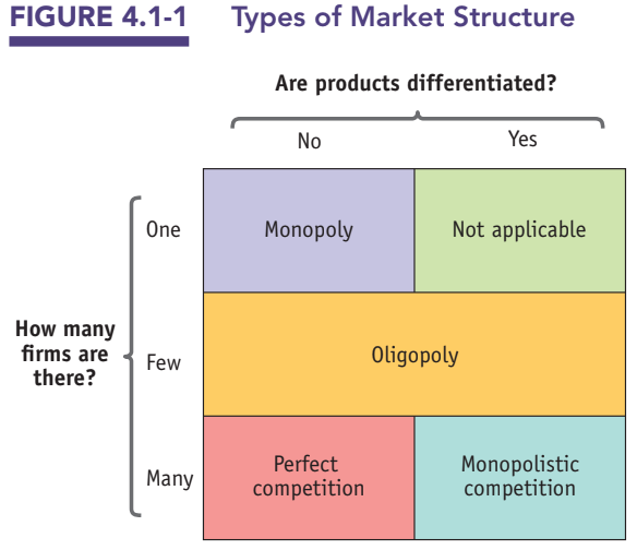
Market structure is determined by two variables: the number of firms in the industry and whether their products are identical (standardized/homogeneous) or differentiated. The two variables generate four combinations, which are the four market structures the AP exam asks about: perfect competition, monopolistic competition, oligopoly, and monopoly.
A monopoly is the extreme case of market power — a single firm is the only producer of a good that has no close substitutes. When De Beers controlled virtually all of the world's diamond production in the 20th century, it was a monopolist. An oligopoly is an industry with only a small number of firms. Even though no single firm has a monopoly, each firm's output decisions noticeably affect market price, and firms must anticipate how rivals will respond. The world banana market, in which three firms produce 65% of output, is an oligopoly. Monopolistic competition combines features of monopoly and perfect competition: many firms compete, each sells a differentiated product, and there is free entry and exit in the long run. The mall food court is the textbook example — each vendor has some monopoly power from its distinctive menu but faces constant competition from the vendor two doors down.
The concentration ratio measures how dominated an industry is by its largest firms. A four-firm concentration ratio of 85%, for instance, means the top four firms account for 85% of sales. Higher concentration generally indicates oligopoly or monopoly; low concentration suggests monopolistic or perfect competition.
The pivotal economic consequence of imperfect competition is the inequality that defines the rest of this unit: P > MC. Because an imperfectly competitive firm faces a downward-sloping demand curve, it must lower price to sell more units — which pulls marginal revenue below price. Setting MR = MC to maximize profit therefore produces a price that exceeds marginal cost. The result is allocative inefficiency: units for which willingness to pay exceeds the cost of production are not produced, so deadweight loss appears.
| Characteristic | Perfect Competition | Monopolistic Competition | Oligopoly | Monopoly |
|---|---|---|---|---|
| Number of firms | Many | Many | Few | One |
| Product type | Identical | Differentiated | Identical or differentiated | Unique |
| Entry barriers | None | None (free entry) | High | Very high |
| Price setting | Price-taker | Some power | Some power | Price-maker |
| Long-run profit | Zero | Zero | Positive possible | Positive |
| Allocatively efficient? | Yes (P = MC) | No (P > MC) | No (P > MC) | No (P > MC) |
Real-World Examples
Which structure does a given industry fit? Here are the canonical examples the AP exam expects you to recognize.
Perfect Competition
- Agricultural commoditiesWheat, corn, soybeans, cotton — thousands of farms, standardized grades, no single seller moves price
- Foreign currency marketsThousands of traders buying/selling identical US dollars; no participant sets the rate
- Fresh-fish auctionsWholesale markets like Tsukiji or Fulton — identical product, posted market price
Monopolistic Competition
- Restaurants & fast foodEvery restaurant has a unique menu; thousands of competitors in any city
- Clothing & apparel brandsLevi's, Gap, Uniqlo, H&M — differentiated by style and brand, easy entry
- Hair salons, coffee shops, gas stationsEach differentiated by location, service, or quality; new entrants constantly
Oligopoly
- Commercial aircraftBoeing and Airbus — a global duopoly; enormous capital barriers
- Smartphones & operating systemsApple, Samsung, Google dominate; network effects + brand barriers
- Soft drinks & auto manufacturersCoke/Pepsi; Ford/GM/Toyota/Honda — few firms, differentiated products, strategic rivalry
- US airlines, wireless carriers, major banks4–6 firms dominating each market; antitrust and regulation keep concentration in check
Monopoly
- Local public utilitiesWater, electricity distribution, natural gas — natural monopolies with regulated prices
- US Postal Service (first-class mail)Government-granted legal monopoly on first-class letter delivery
- Patented pharmaceuticalsDuring the ~20-year patent window, the drug's inventor has sole production rights
- De Beers (historical)Controlled ~90% of world diamond supply through most of the 20th century — the textbook resource monopoly
Monopoly
A monopolist sets its own price. How does it decide how much to produce — and what does that do to total welfare?
Learning Objective
- Identify the types of barriers to entry that allow monopolies to persist.
- Use a graph to show how a profit-maximizing monopolist chooses price and quantity.
- Explain why monopolists charge a price that exceeds marginal cost.
- Calculate consumer surplus, producer surplus, profit, and deadweight loss for a monopoly.
Essential Knowledge
- A monopoly is the sole producer of a good with no close substitutes.
- Barriers to entry: control of resources, economies of scale (natural monopoly), technological superiority (incl. network externalities), government-created barriers (patents, copyrights).
- Monopolist's demand curve is the entire market demand curve — downward-sloping.
- To sell more, the monopolist must lower price; this makes MR < P at every quantity.
- Profit maximization: produce at MR = MC; find price on the demand curve above that quantity.
- Monopoly profit = (Pₘ − ATCₘ) × Qₘ.
- Monopoly creates deadweight loss (DWL) because Qₘ < the socially efficient quantity (where P = MC).
A monopoly is an industry controlled by a single producer selling a good with no close substitutes. For a monopoly to persist, something must prevent other firms from entering — a barrier to entry. The AP curriculum names four types.
Control of a scarce resource or input: if one firm owns essentially the entire supply of a key input, no one else can produce the good. De Beers achieved this with diamond mines in the 20th century.
Economies of scale: in some industries, average cost falls across the entire range of market demand. One large firm can produce the industry's output at a lower average cost than two or more smaller firms could. This is a natural monopoly — and most public utilities (electricity distribution, water, gas, cable internet) are examples because the fixed cost of laying infrastructure is enormous.
Technological superiority: a firm with technology that competitors cannot replicate can dominate a market. In high-tech industries, this often combines with network externalities — the value of the good to one user rises as more users adopt it. Microsoft Windows, Facebook, and WeChat all benefit from network externalities.
Government-created barriers: a patent grants an inventor exclusive rights to produce or license an invention for a limited period (typically 20 years in the US), creating a legal temporary monopoly. A copyright similarly grants exclusive rights to a literary or artistic work. Both exist to incentivize innovation by letting the creator capture the returns from their work.
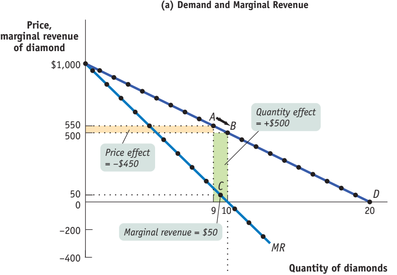
The demand curve a monopolist faces is downward-sloping — it is literally the entire market demand curve. To sell more units, the monopolist must lower price. This is the critical difference from perfect competition. A perfectly competitive firm faces a horizontal demand curve at the market price, so MR = P. A monopolist, however, sees two effects every time it tries to sell one more unit: the quantity effect (one more unit sold at the new, lower price) plus the price effect (every previously sold unit now sells at the lower price). Marginal revenue is the sum of these two effects, and because the price effect is negative, MR < P at every quantity.
Consider De Beers facing a demand of Q = 20 − P/50. At Q = 9, price = $550 (point A), so total revenue is $4,950. To sell a 10th diamond, price must drop to $500 for all 10 diamonds (point B). The quantity effect adds $500 (the 10th unit at $500); the price effect subtracts $450 (9 original units × $50 price cut). Net marginal revenue is $50 — far below the price of $500. Mathematically, if demand is P = a − bQ (linear), MR = a − 2bQ, so MR has twice the slope of demand.
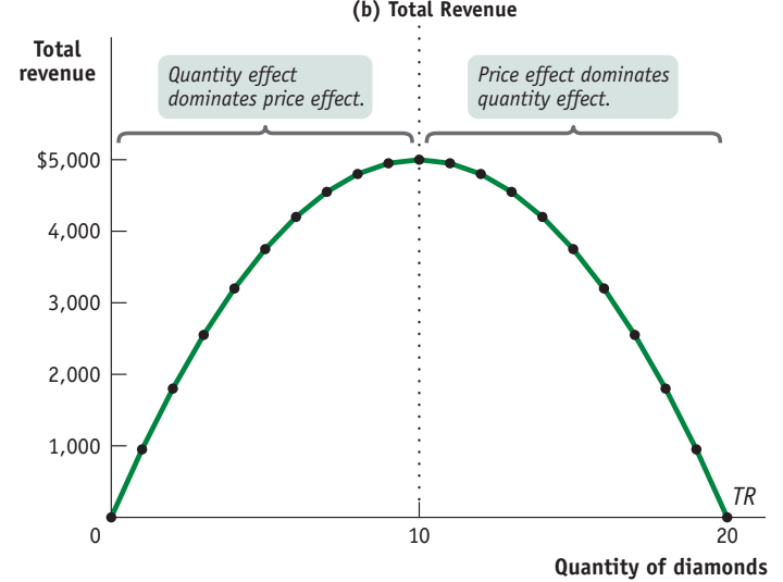
The complete demand schedule for De Beers diamonds appears in Table 4.2-1. Column 1 is the price (P), Column 2 is the quantity demanded at that price (Q), Column 3 is total revenue (TR = P × Q), and Column 4 is marginal revenue (MR = ΔTR/ΔQ) — the change in total revenue when one more diamond is sold. Notice: MR is less than price at every quantity, TR peaks at $5,000 when Q = 10, and MR turns negative beyond that. The highlighted rows (Q = 9 → Q = 10) show the exact move illustrated in Figure 4.2-2(a) below.
| Price of diamond P |
Quantity demanded Q |
Total revenue TR = P × Q |
Marginal revenue MR = ΔTR / ΔQ |
|---|---|---|---|
| $1,000 | 0 | $0 | — |
| $950 | 1 | $950 | $950 |
| $900 | 2 | $1,800 | $850 |
| $850 | 3 | $2,550 | $750 |
| $800 | 4 | $3,200 | $650 |
| $750 | 5 | $3,750 | $550 |
| $700 | 6 | $4,200 | $450 |
| $650 | 7 | $4,550 | $350 |
| $600 | 8 | $4,800 | $250 |
| $550 | 9 | $4,950 | $150 |
| $500 | 10 | $5,000 | $50 |
| $450 | 11 | $4,950 | −$50 |
| $400 | 12 | $4,800 | −$150 |
| $350 | 13 | $4,550 | −$250 |
| $300 | 14 | $4,200 | −$350 |
| $250 | 15 | $3,750 | −$450 |
| $200 | 16 | $3,200 | −$550 |
| $150 | 17 | $2,550 | −$650 |
| $100 | 18 | $1,800 | −$750 |
| $50 | 19 | $950 | −$850 |
| $0 | 20 | $0 | −$950 |
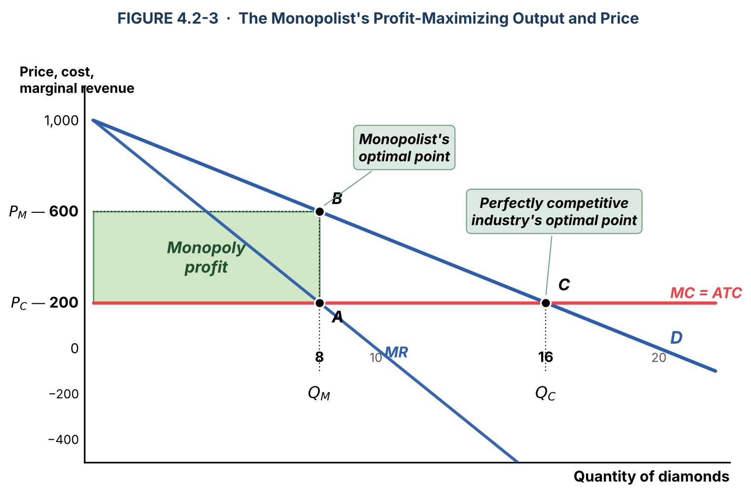
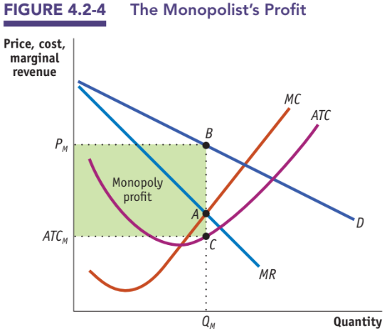
The profit-maximizing rule MR = MC applies to a monopolist just as it does to a perfect competitor — but with one twist. Because MR < P for a monopolist, the price it charges is not the MC value found at the intersection. Instead, after locating the quantity Qₘ where MR = MC (point A), the monopolist slides straight up to the demand curve to find Pₘ (point B). The height of ATC at Qₘ is C, and economic profit is the rectangle with width Qₘ and height (Pₘ − ATCₘ).
The result: compared to a perfectly competitive industry producing the same product with the same cost structure, the monopolist (1) produces less (Qₘ < Qc), (2) charges more (Pₘ > Pc), and (3) earns positive economic profit that persists in the long run because entry is blocked.
Before looking at the general U-shaped-ATC picture, work through the simplest textbook case: constant MC = ATC = $200. This is the De Beers example with no fixed costs — all costs are per-unit. Figure 4.2-3 shows the whole picture on one graph: the monopolist's optimum at point A (Q = 8, where MR = MC), the price read from demand at point B (Pₘ = $600), and the perfectly competitive outcome at point C (Q = 16, P = $200, where D crosses MC). The green rectangle is monopoly profit = ($600 − $200) × 8 = $3,200. Compared to perfect competition, the monopoly produces half as much and charges three times the price.
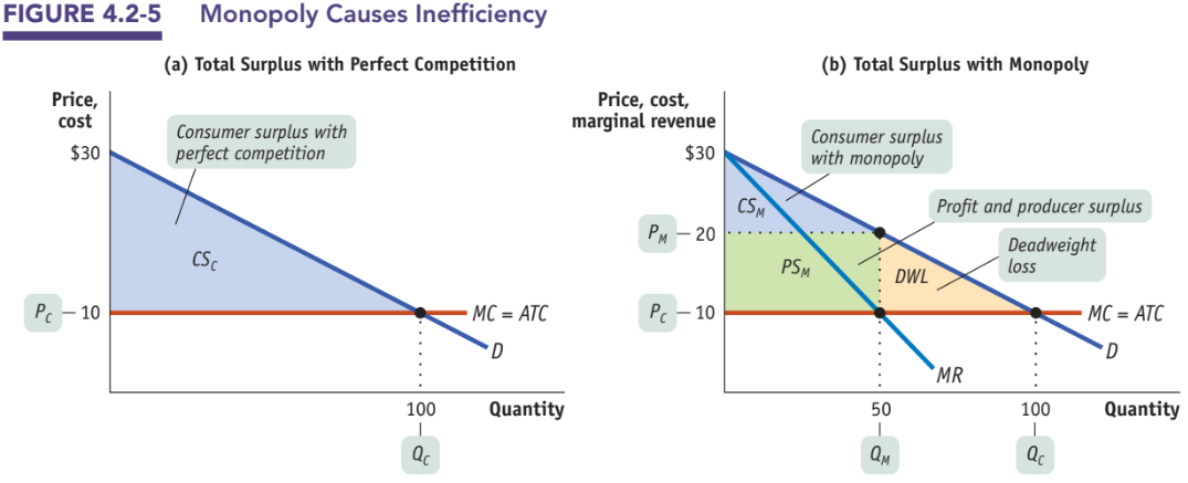
Monopoly is not just a transfer of surplus from consumers to the monopolist — it is a net loss for society. Panel (a) shows the perfectly competitive outcome: price Pc, quantity Qc, consumer surplus is the full triangle under the demand curve above Pc, producer surplus is the triangle between MC and Pc. Panel (b) shows the monopoly outcome: Qₘ is smaller, Pₘ is higher. Consumer surplus (blue) shrinks dramatically. The green rectangle (and the triangle beneath it) is producer surplus — most of it is pure profit. The yellow triangle between Qₘ and Qc, bounded above by demand and below by MC, is deadweight loss. Those are the trades that would have happened under perfect competition but don't under monopoly — buyers whose willingness to pay exceeded MC but who no longer get to buy at the higher Pₘ.
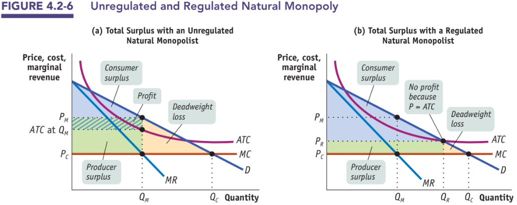
What should policy do? For most monopolies, the answer is antitrust policy — prevent monopoly formation, break up existing monopolies, or regulate conduct. For natural monopolies (where high fixed costs make a single producer the lowest-cost option), breaking the firm into competitors would just raise average costs for everyone. The two main policy responses are: public ownership (the government owns the firm, like USPS or many foreign utilities), and price regulation — the regulator caps the price. The textbook regulated price is where P = ATC (so-called "fair return" pricing): the firm earns zero economic profit while quantity expands beyond Qₘ. The socially efficient regulated price is P = MC, but that would force the firm into losses whenever ATC > MC — a problem for any natural monopoly whose ATC is still falling.
Price Discrimination
Why does the person next to you on the plane almost certainly pay a different price for the same seat?
Learning Objective
- Define price discrimination and distinguish it from a single-price monopoly.
- Explain why price discrimination allows a monopolist to capture additional consumer surplus.
- Show how perfect price discrimination eliminates deadweight loss.
Essential Knowledge
- A single-price monopolist charges every buyer the same price.
- A firm engages in price discrimination when it charges different prices to different buyers for the same good.
- Price discrimination requires: (1) market power, (2) ability to distinguish buyers by willingness to pay, and (3) ability to prevent resale.
- Buyers with more inelastic demand are charged higher prices; more elastic buyers get lower prices.
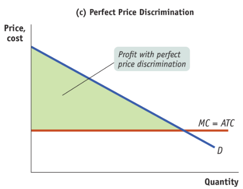
- Under perfect price discrimination, each buyer is charged exactly their willingness to pay — consumer surplus = 0 and DWL = 0 (all of it becomes profit).
A single-price monopolist charges the same price to every customer, as the graphs in 4.2 assumed. But many monopolists (and many non-monopolists with some market power) can do better by charging different prices to different buyers for the same product — the practice known as price discrimination. Three conditions must hold for a firm to price-discriminate successfully: (1) it must have some market power (price-takers cannot discriminate), (2) it must be able to distinguish buyers who have different willingness to pay, and (3) it must be able to prevent resale from low-price buyers to high-price buyers.
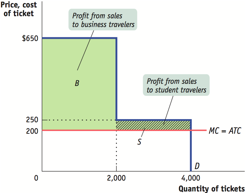
Consider Air Sunshine, which serves 2,000 business travelers (willing to pay up to $650 per ticket) and 2,000 students (willing to pay up to $250). Marginal cost per seat is $200. If Air Sunshine must charge a single price, it must choose between $650 (serves only business, earns 2,000 × $450 = $900,000) and $250 (serves everyone, earns 4,000 × $50 = $200,000). It picks $650 and leaves the student market unserved. If it can distinguish the two groups — say, by requiring students to show ID or by selling tickets through different channels — it can charge $650 to business travelers and $250 to students, earning $900,000 + $100,000 = $1,000,000. The student market is served, and total surplus rises.
In practice, airlines rarely charge different fares by group label (which is often illegal). Instead they design pricing mechanisms that sort customers by willingness to pay. The AP exam names three common techniques:
Advance-purchase restrictions: tickets bought weeks in advance cost less than tickets bought the day before departure. Business travelers (less price-sensitive, book last-minute) pay more; leisure travelers (more price-sensitive, book early) pay less.
Volume discounts: lower per-unit price for buyers purchasing in bulk. Buyers of large quantities tend to be more price-sensitive than one-off shoppers.
Two-part tariffs: a fixed membership or access fee plus a per-unit price (Costco's annual membership plus item prices). The fixed fee captures consumer surplus from heavy users without pricing out light users.
The general principle: more price-elastic buyers get lower prices, less elastic buyers get higher prices. This matches the inverse elasticity rule of monopoly pricing — markups should be larger where elasticity is smaller.
The extreme case is perfect price discrimination: the monopolist charges each buyer exactly their willingness to pay — not a penny more and not a penny less. The firm then produces every unit for which willingness to pay ≥ MC — exactly the socially efficient quantity. There is no consumer surplus (every buyer pays their maximum) and no deadweight loss (every mutually beneficial trade occurs). The entire area between the demand curve and MC becomes profit.
This is a famous exam trap: perfect price discrimination is allocatively efficient (Q = Qc, no DWL) even though it is also maximally unequal (all surplus goes to the firm). Students often check "efficient = fair" — be careful: price discrimination transfers surplus, it doesn't destroy it.
Monopolistic Competition
Many small competitors, each with a slightly distinct product. What outcome does free entry produce?
Learning Objective
- Determine price and profit for a monopolistically competitive firm in both the short run and the long run.
- Explain how free entry drives economic profit to zero in long-run equilibrium.
- Explain why monopolistic competition leads to excess capacity and allocative inefficiency.
- Discuss advertising and product differentiation as competitive tools.
Essential Knowledge
- Monopolistic competition: many firms, differentiated products, free entry and exit.
- Each firm faces a downward-sloping demand curve → MR < P → profit max at MR = MC.
- Short run: a firm may earn positive, zero, or negative economic profit.
- Long run: entry (if profit) or exit (if loss) shifts each firm's D until D is tangent to ATC at the profit-maximizing quantity → zero economic profit.
- At the long-run equilibrium: P > MC (allocatively inefficient) and Q < min-ATC quantity (excess capacity).
- Firms differentiate by style/type, location, and quality, and compete through advertising and brand names.
Monopolistic competition is the hybrid market structure in which many firms sell differentiated versions of a similar product with free entry and exit. The food court, hair salons, independent coffee shops, and gas stations are all canonical examples. Each firm has some monopoly power — your haircut from stylist A is not literally the same as your haircut from stylist B — so each firm faces a downward-sloping demand curve. But because there are many near-substitute options, that demand curve is relatively elastic, and new firms can enter easily.
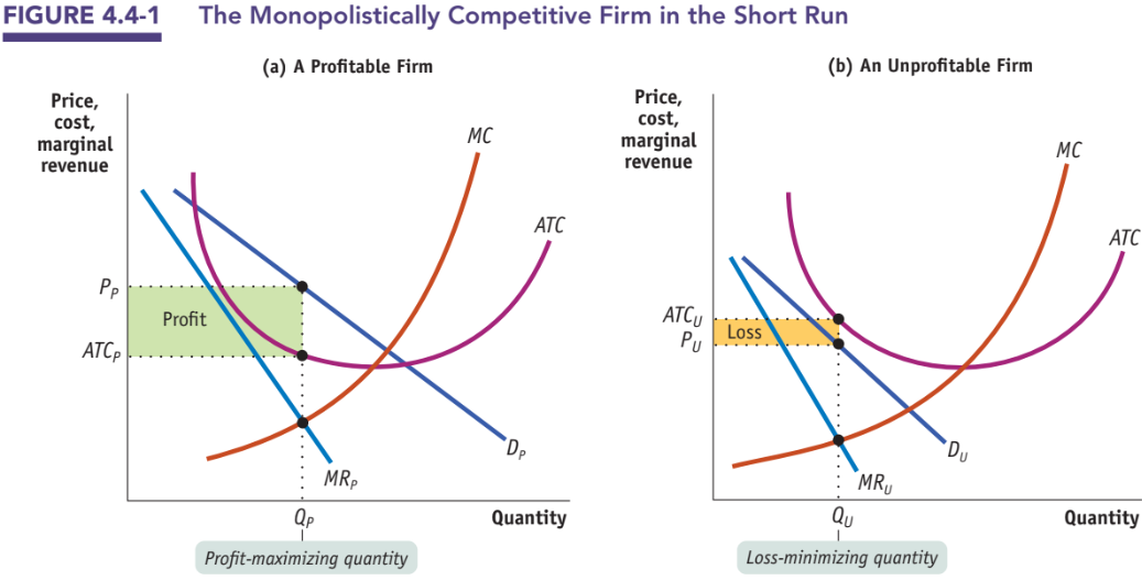
In the short run, a monopolistically competitive firm behaves exactly like a mini-monopoly: it finds Q where MR = MC, charges P on its demand curve above Q, and compares P to ATC to determine profit or loss. If the firm's demand (Dₚ) sits above ATC at the profit-maximizing quantity, it earns a positive economic profit (green rectangle). If the firm's demand (Dᵤ) lies entirely below ATC — meaning no price yields non-negative profit — it operates at a loss (orange rectangle), minimizing the loss by producing at MR = MC where loss is smallest.
The long run is where monopolistic competition differs sharply from pure monopoly. Because entry is free, positive economic profit attracts new firms. New entrants poach customers from existing firms, which shifts each existing firm's demand curve to the left (and MR with it). Symmetrically, losses cause exit — each remaining firm's demand shifts rightward. Figure 4.4-2 shows both mechanisms.
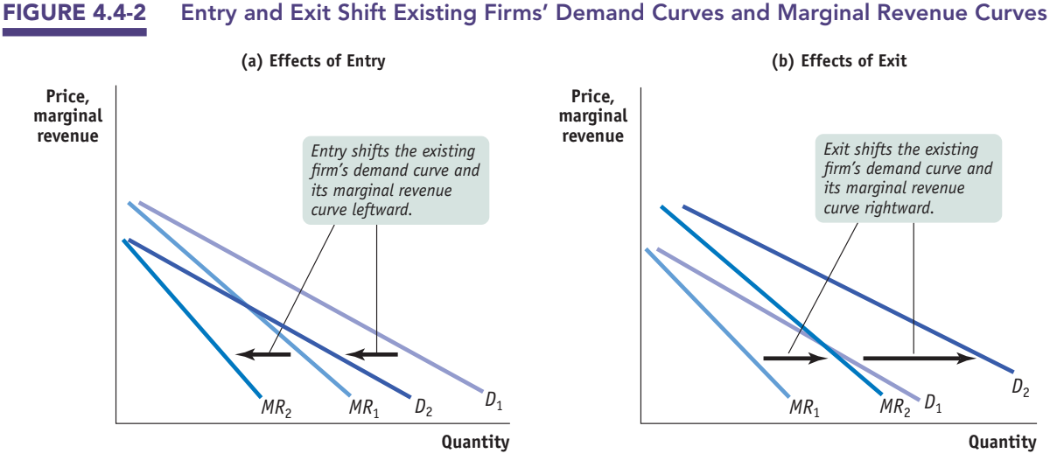
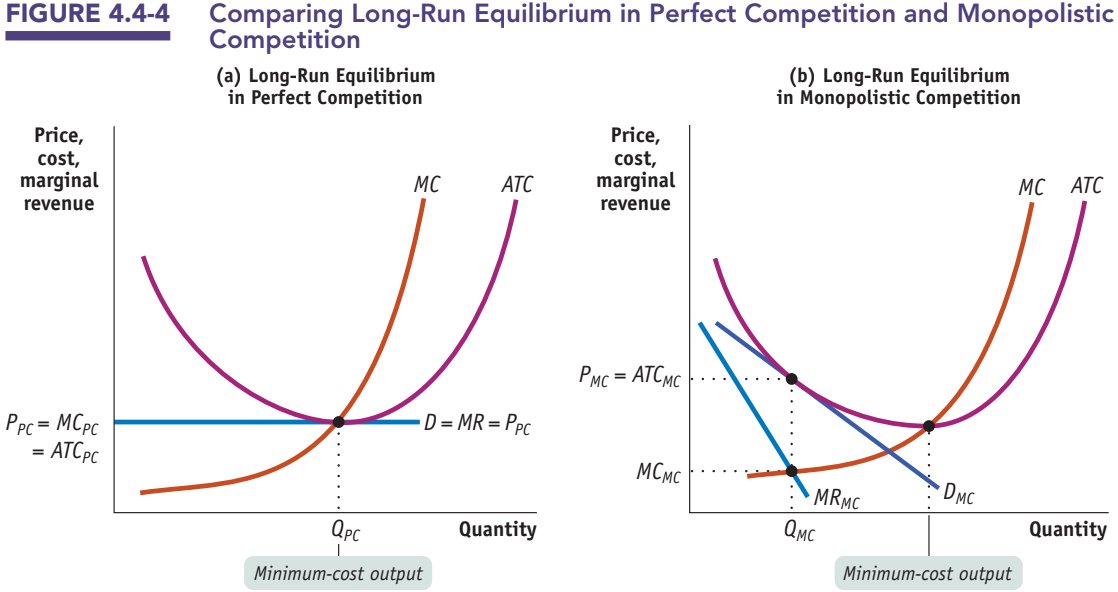
Entry continues until the typical firm's demand curve has shifted all the way down to be tangent to its ATC curve at the profit-maximizing quantity. At that tangency point: Pₘc = ATCₘc, so economic profit = 0. Exit works the same way in reverse: it stops once losses are eliminated and each remaining firm earns zero economic profit.
Long-run equilibrium under monopolistic competition therefore has two defining features:
First, zero economic profit: free entry and exit force the long-run tangency of D with ATC. Firms in monopolistic competition cannot earn positive economic profit in the long run, just like firms in perfect competition.
Second, allocative inefficiency and excess capacity: because the firm faces a downward-sloping D, the tangency with ATC must occur on the left (downward-sloping) portion of ATC, not at the minimum. So at the profit-maximizing quantity Qₘc, two things are true: P > MC (allocatively inefficient — same P > MC story as monopoly), and Qₘc < the min-ATC quantity, which is called excess capacity. The firm is operating at a point where producing more would lower its average cost.
Why do firms in monopolistic competition try so hard to differentiate their products? Because differentiation is what preserves the downward slope of their demand curve — the only thing that gives them any pricing power. The AP curriculum identifies three forms of product differentiation:
Differentiation by style or type: a Thai food stall and a burger stall at the food court sell imperfect substitutes — some diners strongly prefer one over the other. Differentiation by location: the gas station just off the freeway exit charges more than the one two miles into town. Differentiation by quality: consumers may be willing to pay more for a product they believe is of higher quality, whether or not it objectively is.
Firms reinforce these differences with advertising and brand names. Advertising serves two economic functions: direct information (announcing a product's features) and indirect signaling (large ad budgets signal that the firm is confident enough in its product to spend heavily). Brand names create recognition that reduces consumer search costs — but also allow firms to charge brand premiums over generic substitutes.
Is monopolistic competition a problem? Economists are split. On one hand, excess capacity and P > MC create deadweight loss just like monopoly does. On the other hand, consumers value variety — the fact that there are 15 types of toothpaste rather than one has real welfare benefits that the standard surplus analysis ignores. The AP exam position is that long-run monopolistic competition is allocatively inefficient (P > MC) and productively inefficient (Q < min ATC) — but may still be the best market structure available when products are naturally varied.
Oligopoly and Game Theory
A handful of firms, each watching every move the others make. What does rational strategy look like?
Learning Objective
- Explain how oligopolists are interdependent and why they have incentives to collude.
- Analyze two-player games using payoff matrices.
- Identify dominant strategies and Nash equilibria.
- Explain how repeated interaction can sustain tacit collusion.
Essential Knowledge
- Oligopolists are interdependent: each firm's profit depends on rivals' actions.
- Collusion: firms coordinate to raise joint profit. A cartel is a formal collusive agreement.
- Noncooperative behavior: each firm acts in its own self-interest.
- A payoff matrix shows every player's payoff for every combination of actions.
- A dominant strategy is a player's best action regardless of what others do.
- A Nash equilibrium is an outcome where no player can improve their payoff by changing strategy, given the others' choices. A game may have 0, 1, or multiple NE.
- The prisoner's dilemma: a game where (a) each player has a dominant strategy to defect, but (b) both playing their dominant strategy yields a worse outcome than mutual cooperation would.
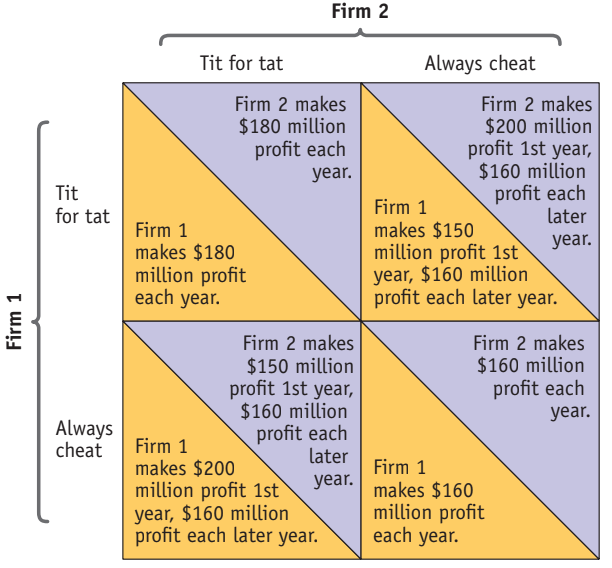
- Tit-for-tat in repeated games can sustain tacit collusion by rewarding cooperation and punishing defection.
An oligopoly is an industry dominated by a small number of firms. The defining feature is interdependence: because each firm's output or pricing decision noticeably affects the market, each firm must anticipate how the others will react. In perfect competition, no firm is big enough to matter. In monopoly, there is no rival to worry about. In oligopoly, every move invites a counter-move — and that is why oligopoly analysis uses game theory: the formal study of strategic decisions under interdependence.
The simplest case is a duopoly — two firms. Consider two developers selling essentially identical dictionary apps. If they collude and both charge the monopoly price of $6, they jointly earn $36 million. If one cheats and undercuts to $5, the cheating firm captures the whole market and the loyal firm earns nothing. If both cheat down to $5, they split the enlarged market but earn far less than they would have under collusion. The four outcomes form a payoff matrix with exactly the structure of the prisoner's dilemma.
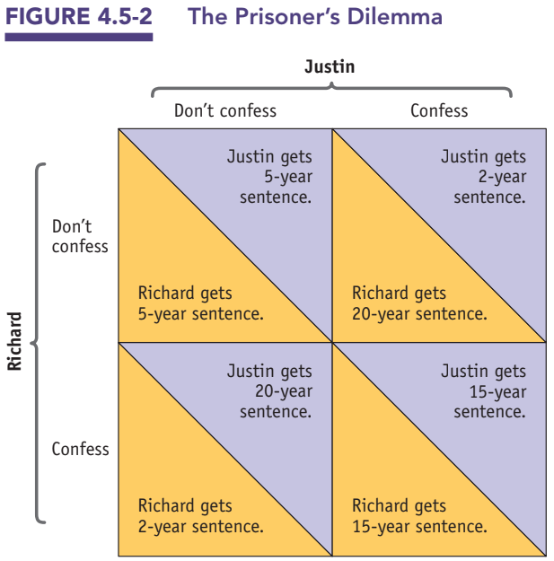
The logic: each suspect reasons, "If the other stays silent, confessing cuts my sentence from 5 years to 2. If the other confesses, confessing cuts my sentence from 20 years to 15. Either way, confess." Confess is a dominant strategy — strictly better regardless of what the other does. Both confess; both get 15 years. The outcome is a Nash equilibrium: given the other's choice to confess, neither can improve by changing. Yet both would prefer the (Don't confess, Don't confess) outcome. That is the prisoner's dilemma: dominant-strategy play is worse for both players than mutual cooperation.
The duopolist's situation is identical. "Collude" plays the role of "Don't confess"; "Cheat" plays the role of "Confess." The one-shot Nash equilibrium is both firms cheating — exactly the structure above.
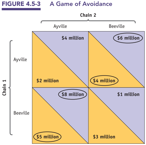
Not every game is a prisoner's dilemma. Nash equilibria can exist without any dominant strategies, and some games have multiple Nash equilibria. In the game of avoidance below, two chain stores prefer to locate in different towns than compete in the same one. There is no dominant strategy — the best choice depends on what the rival does. There are two Nash equilibria: whichever chain commits first typically picks its preferred town; the other then picks the other town.
The prisoner's dilemma logic suggests that oligopolists should compete away all their joint profit. In practice, they often don't. Why? Because real oligopolists interact repeatedly, not once. The strategy of tit-for-tat — cooperate on the first round, then mimic whatever the rival did last round — rewards sustained cooperation and immediately punishes defection. If both firms expect the other to play tit-for-tat, both can rationally sustain cooperation indefinitely. This is called tacit collusion: firms coordinate on the monopoly outcome without ever meeting to agree.
Several forces push against tacit collusion: (1) antitrust laws make explicit collusion illegal and tacit collusion risky; (2) the more firms in the industry, the harder it is for all of them to coordinate; (3) complex products and pricing make it hard to tell whether a rival is cheating; and (4) differences in firm interests (different cost structures, different market shares) make the "fair" cooperative price hard to agree on.
Sources & Further Reading
- College Board — AP Microeconomics Course and Exam Description, Unit 4: Imperfect Competition.
- Krugman & Wells, Microeconomics for the AP Course, 4th ed. (BFW Publishers, 2023), Modules 4.1–4.5.
- Khan Academy Microeconomics — Monopoly, Price Discrimination, Monopolistic Competition, Oligopoly units.
- Mankiw, Principles of Microeconomics, Chapters 15–17.
- Nash, J. F. (1950). "Equilibrium Points in n-Person Games." Proc. Natl. Acad. Sci. 36(1): 48–49.