Production, Cost & Perfect Competition

A production function is the relationship between the quantity of inputs a firm uses and the quantity of output it produces. Every firm — from a wheat farmer to a tech company — has one. Inputs come in two flavors: a fixed input is one whose quantity cannot be varied over some period of time (typically capital, land, or a factory building), and a variable input is one whose quantity the firm can adjust at any time (typically labor, raw materials, or energy). Whether an input is fixed depends entirely on the time horizon.

This gives rise to the crucial distinction between short run and long run. The short run is any time period in which at least one input is fixed. The long run is a period long enough that all inputs become variable — the firm can build a new factory, sign a new lease, buy new equipment. Note that the short run and long run don't refer to any predetermined amount of clock time; they are defined by which inputs are variable.

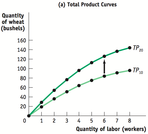
In the short run, with capital fixed, the firm can only expand output by adding more labor. The total product curve (TP) shows this graphically: as more workers are added to the fixed capital stock, total output rises but at a decelerating rate. It slopes upward because more labor produces more wheat, but it becomes flatter because the marginal product of each additional worker declines.

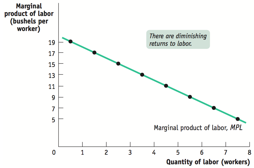
The marginal product of labor (MPL) is the additional output produced by hiring one more worker: MPL = ΔTP / ΔL. Because of the declining slope of the TP curve, the MPL curve slopes downward — this is the law of diminishing marginal returns. Each new worker added to a fixed amount of land (or capital) contributes less to total output than the previous worker. On Mia and Liam's farm, for example, the first worker might add 19 bushels, the second 17, the third 15, and so on. The first worker has all the land and tools to themselves; the tenth worker is crowding into the same fixed space.

Sometimes the first few workers can actually raise each other's productivity through specialization — one plants, another waters, another harvests. In that case MPL rises initially before eventually falling. But sooner or later, diminishing returns must set in, because the fixed input becomes the bottleneck.

Alongside marginal product, we track average product (AP): the total output divided by the quantity of the variable input (AP = TP/L). This is the output per worker on average. The relationship between MP and AP is purely mathematical — the same "test score" logic that will show up again in cost curves later. Whenever a new worker's contribution (MP) exceeds the current average (AP), it pulls the average up: if MP > AP, then AP is rising. Whenever a new worker's contribution falls short of the average, it pulls the average down: if MP < AP, then AP is falling. The two curves cross precisely at AP's maximum: MP = AP at the peak of AP. This is not a coincidence — it's the same reason a test score above your average raises your GPA, and one below it drags your GPA down.

What happens when the fixed input itself changes? If the farm expands from 10 acres to 20 acres, each worker now has more land to work with, and the marginal product of each worker rises. Graphically, the entire TP curve shifts up (from TP₁₀ to TP₂₀) and the entire MPL curve shifts up (from MPL₁₀ to MPL₂₀). Both curves still slope in their usual directions — TP still curves down, MPL still slopes downward — but at every level of labor, output and marginal product are higher when there is more land.

Every cost curve in the short run derives directly from the production function. A fixed cost (FC) is the cost of the fixed input — it does not depend on the quantity of output. Whether Selena's Gourmet Salsas produces 1 case or 100 cases per day, the daily rent on her food-preparation equipment ($108) is the same. A variable cost (VC) is the cost of the variable input — it rises as output rises because more workers, more jars, and more ingredients are needed. Total cost is simply the sum: TC = FC + VC.

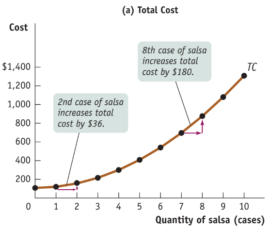
The total cost curve slopes upward because more output requires more workers and more materials. It also becomes steeper as output rises, and that steepness reflects diminishing marginal returns to labor: as more workers are added to the fixed equipment, each additional case of salsa requires disproportionately more labor. Marginal cost (MC) is the change in total cost from producing one more unit — geometrically, it is the slope of the total cost curve. Because TC steepens with output, MC rises with output (in the simplest model).

Once we start dividing costs by quantity, we get the "average" family of curves. Average fixed cost (AFC = FC/Q) falls continuously, because we're spreading a fixed number over a bigger and bigger denominator — this is called the spreading effect. Average variable cost (AVC = VC/Q) eventually rises because of diminishing returns — this is the diminishing returns effect. Average total cost (ATC = TC/Q = AFC + AVC) is the sum of the two.

The U-shape of ATC is a tug-of-war between these two forces. At low output, the spreading effect dominates (AFC is falling fast) and ATC falls. At high output, diminishing returns dominate (AVC is rising fast) and ATC rises. The bottom of the U is the minimum-cost output — the quantity at which average total cost is lowest.

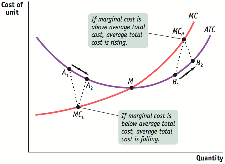
The single most-tested relationship in this topic: MC always crosses ATC (and AVC) at their minimum points. This is a mathematical necessity, not a coincidence. Whenever MC < ATC, each new unit is cheaper than the current average, pulling the average down. Whenever MC > ATC, each new unit is more expensive than the average, pulling it up. So ATC can only be at its minimum precisely when MC = ATC. The same logic applies to AVC.

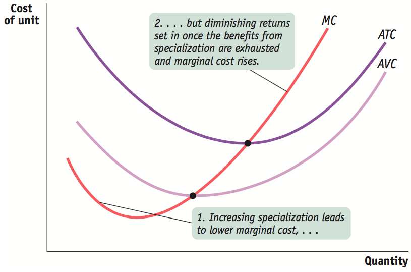
The real-world MC curve often has a "swoosh" shape rather than being uniformly upward-sloping. At very low output, adding the first few workers lets them specialize, which raises MP and lowers MC. Once specialization is exhausted, diminishing returns take over and MC turns upward. In this more realistic setup, both MC and AVC are U-shaped, and MC still intersects AVC at its minimum.

In the short run, a firm is stuck with a fixed capital stock — a given factory. If it wants to produce more, it can only add labor to that fixed plant. In the long run, however, all costs become variable: leases expire, equipment can be sold or bought, factories can be built or closed. Selena can choose to buy more food-preparation equipment, which will raise her fixed cost but lower her variable cost per case (since fewer workers will be needed).

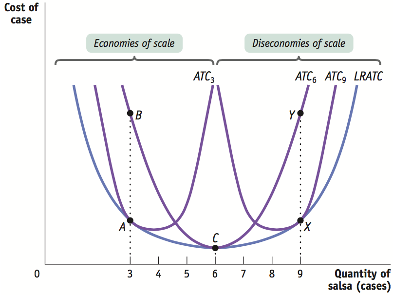
There is always a trade-off between higher fixed cost and lower variable cost, and vice versa. If Selena expects to produce only 3 cases per day for a long time, she should choose a small plant with low fixed cost. If she expects to produce 9 cases per day, a bigger plant with higher fixed cost but lower per-unit variable cost is optimal. Each short-run ATC curve (ATC₃, ATC₆, ATC₉) corresponds to one particular plant size.

The long-run average total cost curve (LRATC) is what you get when you pick the best (cost-minimizing) plant for every possible output level — the lower boundary, or "envelope," of all those short-run curves. Each SRATC is tangent to the LRATC at exactly one point: the output for which that plant size is optimal.

The shape of the LRATC is determined by returns to scale. When output rises more than in proportion to inputs (doubling inputs more than doubles output), the firm has increasing returns to scale, and LRATC falls — this is economies of scale, driven by specialization, division of labor, bulk discounts, and more efficient large-scale technology. When output rises less than in proportion to inputs (doubling inputs less than doubles output), the firm has decreasing returns to scale, and LRATC rises — this is diseconomies of scale, driven by coordination failures, management layers, and communication bottlenecks. When output rises exactly in proportion to inputs, the firm has constant returns to scale, and LRATC is flat.

The minimum efficient scale (MES) is the smallest quantity at which LRATC is minimized. It matters enormously for market structure. If MES is large relative to total market demand, only a few large firms can survive — the industry tends toward oligopoly or monopoly. If MES is small, many small firms can coexist — the industry is competitive.

Important distinction: diminishing marginal returns is a short-run concept — it depends on having a fixed input. Returns to scale is a long-run concept — all inputs are variable. Do not conflate them.

The primary goal of most firms is to maximize profit — but the definition of profit depends on who is measuring it. Accountants and economists count costs differently, and that difference matters for real decisions.

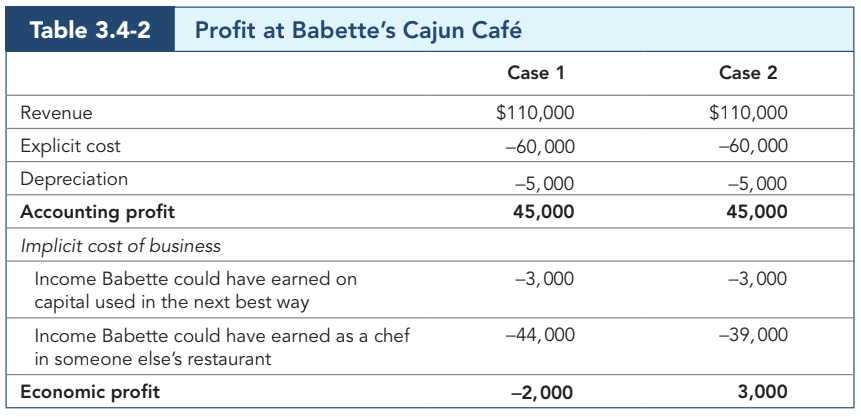
An explicit cost is a cost that involves actually laying out money — cash paid to workers, suppliers, landlords, and utility companies. An accountant records only these out-of-pocket expenditures. An implicit cost does not require any outlay of money; it is the value, in dollar terms, of benefits that are forgone. If Babette owns her restaurant building instead of renting it out, there is no rent check to record, but she is still giving up the rental income the building could have earned. That forgone income is a real implicit cost of running the restaurant.

For students, the biggest implicit cost is often the value of time itself. The time spent on any activity is an implicit cost equal to the next-best alternative use of that time. College students incur not only explicit costs like tuition, but also the implicit cost of forgone income from the job they aren't holding while studying.

Accounting profit = Total Revenue − Explicit Costs − Depreciation. This is what appears on financial statements. Economic profit = Total Revenue − Explicit Costs − Implicit Costs. Because implicit costs are always ≥ 0, economic profit is always ≤ accounting profit.

This gives rise to a critical concept: normal profit — an economic profit exactly equal to zero. A firm earning normal profit is covering all of its explicit costs and all of its implicit costs. All resources earn exactly what they could earn in their next-best alternative use. There is no incentive to enter or exit the industry. Normal profit is the "just enough to stay" condition and is the long-run equilibrium target in perfectly competitive markets.

When a firm earns positive economic profit (above-normal), it is earning more than all inputs could earn elsewhere — new firms are attracted and entry occurs. When economic profit is negative (below-normal, or an economic loss), resources could do better elsewhere and exit occurs. Only at zero economic profit does the market reach a stable long-run equilibrium. A firm with normal profit (zero economic profit) may still show positive accounting profit — because accountants ignore implicit costs.

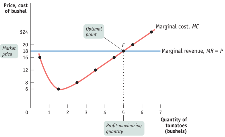
The principle of marginal analysis says that every activity should continue up to the point where marginal benefit equals marginal cost. Applied to a firm's output decision: marginal revenue (the extra revenue from selling one more unit) is the marginal benefit of producing, and marginal cost is the marginal cost of producing. Combine them and you get the profit-maximizing rule (or "optimal output rule"): produce the quantity at which MR = MC.

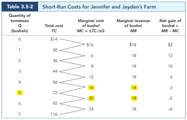
Every unit where MR > MC adds to total profit — so produce it. Every unit where MR < MC subtracts from total profit — so don't produce it. The profit-maximizing firm therefore stops precisely at MR = MC. This rule holds for every market structure; what changes between structures is the relationship between marginal revenue and price.

In a perfectly competitive market, each firm is a price taker: it can sell any quantity at the market price P but nothing above it. Every additional unit adds exactly P to revenue, so MR = P. The firm's individual demand curve is therefore a horizontal line at the market price. The firm simply finds where this price line crosses its MC curve — that is the profit-maximizing output Q*.

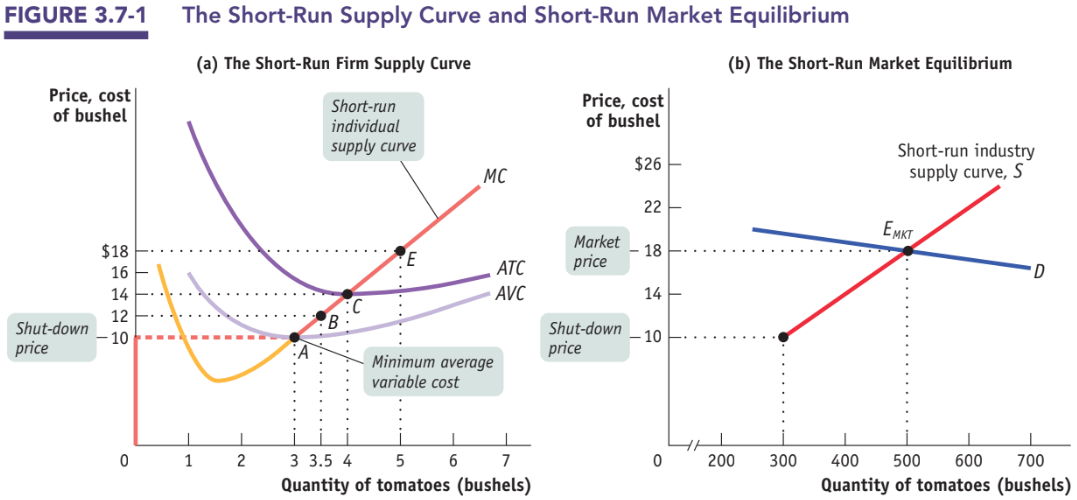
Consider Jennifer and Jayden selling bushels of organic tomatoes for $18 each. Because MR = $18 for every bushel, they should keep adding bushels as long as MC ≤ $18. At 5 bushels, MC = $16 (still less than MR = $18, so produce it). At 6 bushels, MC would rise to $22 (greater than MR = $18, so don't produce it). The profit-maximizing quantity is 5 bushels — the last one at which MC ≤ MR.

To find the profit or loss, compare P to ATC at Q*. If P > ATC, the firm earns economic profit — a rectangle with height (P − ATC) and base Q*. If P = ATC, the firm breaks even (normal profit). If P < ATC but P > AVC, the firm operates at a loss but keeps running in the short run because it covers its variable costs and part of its fixed costs. If P < AVC, the firm shuts down (covered in 3.6).

A firm should stay in business, in the long run, if selling its optimal quantity at the market price results in at least a normal profit — that is, economic profit ≥ 0. In the short run, however, the criterion is different because fixed costs are unavoidable (again, see 3.6).

A perfectly competitive firm follows MR = MC to find its optimal output. But whether that optimum yields a profit, a loss, or exactly zero economic profit depends on where the market price sits relative to the firm's cost curves.

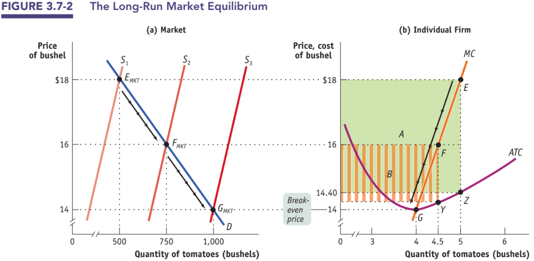
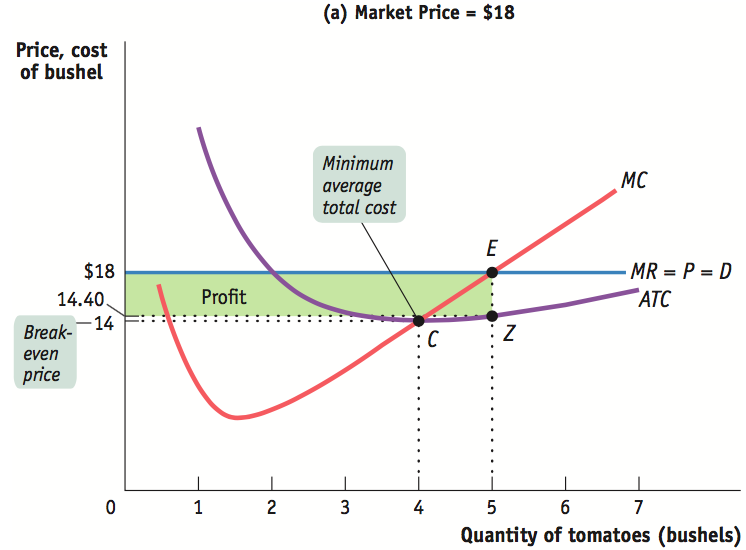
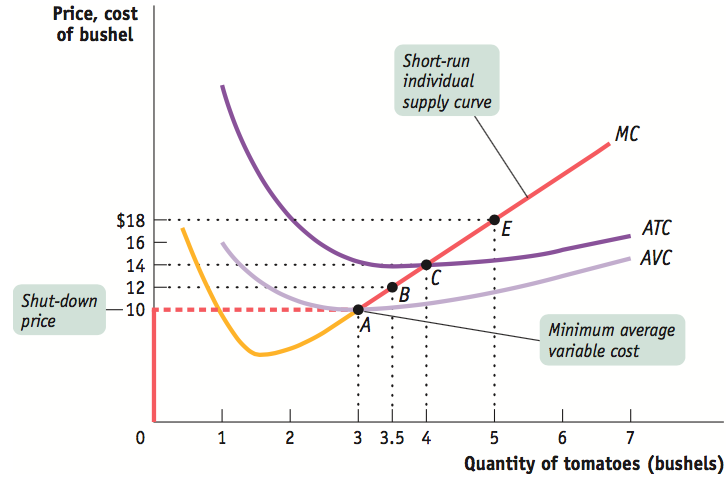
When the market price is above the firm's minimum ATC, the firm is profitable. If P = $18 exceeds the firm's minimum ATC of $14, Jennifer and Jayden's farm produces the optimal 5 bushels (where MR = MC at point E). At that quantity, ATC = $14.40 (shown by point Z on the ATC curve). Per-unit profit is P − ATC = $18.00 − $14.40 = $3.60, and total profit is (P − ATC) × Q = 5 × $3.60 = $18. This is drawn as a green rectangle between P and ATC.

When the market price falls below minimum ATC, the firm operates at a loss. If P drops to $10, the optimal output falls to 3 bushels (where the new MR = MC), and ATC at that quantity is $14.67. Per-unit loss = $14.67 − $10 = $4.67, total loss ≈ $14 (shown as an orange rectangle above P and below ATC).

Now the crucial question: should a losing firm keep producing? The insight is that fixed costs are unavoidable in the short run — the tomato farmer pays for the tractor lease whether or not they plant tomatoes. So the relevant short-run comparison is variable cost vs. revenue, not total cost vs. revenue. If the price at least covers AVC, operating is better than shutting down, because the firm recovers something toward the fixed costs it owes anyway.

The shutdown rule: if P ≥ min AVC, produce at MR = MC (even at a loss, if P < ATC). If P < min AVC, shut down and lose only FC. The shut-down price equals min AVC and is where the firm is exactly indifferent between producing and closing temporarily. The break-even price equals min ATC — the price at which the firm earns zero economic profit.

The firm's short-run supply curve is therefore the portion of the MC curve at or above min AVC. Below that shutdown price, the firm produces zero — its supply curve lies along the vertical axis.

In the long run, fixed costs become variable — leases expire, equipment can be sold. Now the relevant comparison is P vs. ATC. A firm persistently earning negative economic profit (P < min ATC) will eventually exit the industry. A firm earning positive economic profit (P > min ATC) invites entry from new competitors. Do not confuse short-run shutdown (stopping production temporarily while still paying FC) with long-run exit (leaving the industry entirely).

Perfect competition is the benchmark market structure — economists don't expect it to exist everywhere, but it defines the ideal outcome against which other structures are compared. A market is perfectly competitive when four conditions hold: many buyers and sellers (no firm has a large market share), a standardized product (buyers view all firms' products as identical), free entry and exit (new firms can join and existing firms can leave without barriers), and full information.

Under these conditions, every firm is a price taker: because products are identical and no seller is big enough to move the market, no individual firm can charge more than the going market price. If it tries, every buyer switches to a competitor instantly. The firm's demand curve is a perfectly horizontal line at P*. Every unit sold earns the same P, so P = MR = AR = D. (A useful mnemonic: MR. DARP for all the curves that overlap this horizontal line — Marginal Revenue, Demand, Average Revenue, Price.)

The short-run industry supply curve is the horizontal sum of the individual firms' supply curves (the MC segments above min AVC). It intersects market demand at the short-run market equilibrium price. In the short run, this price can land anywhere relative to firms' costs, so firms may earn positive economic profit, break even, or operate at a loss.

The long-run adjustment mechanism is what makes perfect competition special. When existing firms earn positive economic profit, that attracts new entrants. The short-run industry supply curve shifts rightward (S₁ → S₂ → S₃), market price falls, and each firm's economic profit erodes. Entry continues until the market price is exactly at min ATC, where economic profit is zero. When existing firms are earning losses, some exit. Supply shifts leftward, market price rises, and the losses shrink until — again — price equals min ATC and firms earn zero economic profit.

At long-run equilibrium, the four-way equality holds: P = MR = MC = min ATC. Firms produce at their most efficient scale, and price equals both the marginal cost of the last unit and the minimum of the average total cost curve. Because P = MC, we have allocative efficiency — each unit produced is worth exactly what it costs society to make. Because P = min ATC, we have productive efficiency — firms use the cheapest available production method. No mutually beneficial trades are left unexploited.

The long-run industry supply curve (LRS) shows the relationship between price and total industry output after all entry/exit adjustments. It is always flatter than the short-run supply curve because firms have more ways to respond. In a constant-cost industry, input prices don't change as industry grows, so LRS is horizontal. In an increasing-cost industry (like cotton, where expansion raises the cost of cotton itself), LRS is upward-sloping. In a decreasing-cost industry, LRS is downward-sloping — expansion actually lowers input costs.